What Kind Of Filter Is Parallel Rlc Circuit

Resistor Inductor Capacitor Circuit

A series RLC network (in order): a resistor, an inductor, and a capacitor

An RLC circuit is an electrical circuit consisting of a resistor (R), an inductor (Fifty), and a capacitor (C), connected in series or in parallel. The proper noun of the circuit is derived from the letters that are used to denote the elective components of this circuit, where the sequence of the components may vary from RLC.

The circuit forms a harmonic oscillator for current, and resonates in a fashion like to an LC excursion. Introducing the resistor increases the decay of these oscillations, which is as well known as damping. The resistor too reduces the peak resonant frequency. Some resistance is unavoidable even if a resistor is not specifically included as a component.

RLC circuits have many applications as oscillator circuits. Radio receivers and tv sets use them for tuning to select a narrow frequency range from ambience radio waves. In this function, the circuit is often referred to as a tuned circuit. An RLC circuit can be used equally a band-pass filter, band-stop filter, low-pass filter or high-laissez passer filter. The tuning application, for example, is an example of band-laissez passer filtering. The RLC filter is described as a 2nd-gild excursion, significant that any voltage or current in the excursion can be described past a second-order differential equation in excursion assay.

The iii circuit elements, R, L and C, can be combined in a number of different topologies. All three elements in serial or all iii elements in parallel are the simplest in concept and the most straightforward to analyse. In that location are, however, other arrangements, some with applied importance in real circuits. One issue oft encountered is the need to take into account inductor resistance. Inductors are typically constructed from coils of wire, the resistance of which is not unremarkably desirable, but information technology often has a meaning effect on the circuit.

Basic concepts [edit]

Resonance [edit]

An important property of this circuit is its ability to resonate at a specific frequency, the resonance frequency, $f 0$ . Frequencies are measured in units of hertz. In this article, angular frequency, $ω 0$ , is used because it is more mathematically user-friendly. This is measured in radians per 2nd. They are related to each other by a simple proportion,

\omega _{0}=2\pi f_{0}\,.

Resonance occurs because energy for this state of affairs is stored in two different ways: in an electric field equally the capacitor is charged and in a magnetic field as current flows through the inductor. Energy can be transferred from 1 to the other within the circuit and this can be oscillatory. A mechanical illustration is a weight suspended on a spring which will oscillate up and downwardly when released. This is no passing metaphor; a weight on a bound is described past exactly the same second order differential equation as an RLC circuit and for all the properties of the ane organization there will be establish an coordinating belongings of the other. The mechanical holding answering to the resistor in the circuit is friction in the leap–weight system. Friction will slowly bring whatsoever oscillation to a halt if in that location is no external force driving it. Besides, the resistance in an RLC excursion volition "damp" the oscillation, diminishing it with time if there is no driving AC power source in the circuit.

The resonance frequency is defined as the frequency at which the impedance of the circuit is at a minimum. Equivalently, it tin can be defined every bit the frequency at which the impedance is purely existent (that is, purely resistive). This occurs because the impedances of the inductor and capacitor at resonance are equal but of opposite sign and cancel out. Circuits where L and C are in parallel rather than series actually have a maximum impedance rather than a minimum impedance. For this reason they are oftentimes described as antiresonators; information technology is still usual, however, to name the frequency at which this occurs as the resonance frequency.

Natural frequency [edit]

The resonance frequency is defined in terms of the impedance presented to a driving source. It is still possible for the excursion to deport on oscillating (for a fourth dimension) afterward the driving source has been removed or information technology is subjected to a step in voltage (including a step down to cipher). This is similar to the way that a tuning fork volition carry on ringing later on it has been struck, and the effect is ofttimes chosen ringing. This issue is the summit natural resonance frequency of the circuit and in general is non exactly the aforementioned as the driven resonance frequency, although the two will commonly exist quite close to each other. Various terms are used by different authors to distinguish the two, merely resonance frequency unqualified usually means the driven resonance frequency. The driven frequency may be chosen the undamped resonance frequency or undamped natural frequency and the peak frequency may exist called the damped resonance frequency or the damped natural frequency. The reason for this terminology is that the driven resonance frequency in a series or parallel resonant circuit has the value^[one]

\omega _{0}={\frac {1}{\sqrt {L\,C~}}}\,~.

This is exactly the aforementioned equally the resonance frequency of an LC circuit, that is, 1 with no resistor nowadays. The resonant frequency for an RLC circuit is the same every bit a circuit in which there is no damping, hence undamped resonance frequency. The elevation resonance frequency, on the other hand, depends on the value of the resistor and is described as the damped resonant frequency. A highly damped circuit will fail to resonate at all when not driven. A circuit with a value of resistor that causes it to be merely on the edge of ringing is called critically damped. Either side of critically damped are described as underdamped (ringing happens) and overdamped (ringing is suppressed).

Circuits with topologies more complex than straightforward series or parallel (some examples described later in the commodity) accept a driven resonance frequency that deviates from $\omega _{0}=1/{\sqrt {Fifty\,C~}}$ , and for those the undamped resonance frequency, damped resonance frequency and driven resonance frequency tin can all be different.

Damping [edit]

Damping is acquired by the resistance in the excursion. It determines whether or not the excursion will resonate naturally (that is, without a driving source). Circuits that will resonate in this fashion are described as underdamped and those that will not are overdamped. Damping attenuation (symbol $α$ ) is measured in nepers per 2d. However, the unitless damping factor (symbol $ζ$ , zeta) is oftentimes a more useful measure, which is related to $α$ by

\zeta ={\frac {\alpha }{\omega _{0}}}\,.

The special case of $ζ = 1$ is called critical damping and represents the example of a circuit that is only on the edge of oscillation. Information technology is the minimum damping that can exist practical without causing oscillation.

Bandwidth [edit]

The resonance outcome can be used for filtering, the rapid change in impedance near resonance can be used to pass or block signals close to the resonance frequency. Both band-pass and ring-stop filters tin can be constructed and some filter circuits are shown later in the article. A fundamental parameter in filter design is bandwidth. The bandwidth is measured between the cutoff frequencies, near often defined as the frequencies at which the power passed through the circuit has fallen to half the value passed at resonance. There are two of these one-half-power frequencies, one above, and one below the resonance frequency

\Delta \omega =\omega _{2}-\omega _{ane}\,,

where $Δ ω$ is the bandwidth, $ω 1$ is the lower half-power frequency and $ω ii$ is the upper half-ability frequency. The bandwidth is related to attenuation by

\Delta \omega =2\blastoff \,,

where the units are radians per second and nepers per second respectively.^{[ citation needed ]} Other units may require a conversion gene. A more general measure of bandwidth is the partial bandwidth, which expresses the bandwidth as a fraction of the resonance frequency and is given by

B_{\mathrm {f} }={\frac {\Delta \omega }{\omega _{0}}}\,.

The fractional bandwidth is also oftentimes stated as a percent. The damping of filter circuits is adapted to result in the required bandwidth. A narrow band filter, such every bit a notch filter, requires depression damping. A broad band filter requires loftier damping.

$Q$ factor [edit]

The $Q$ factor is a widespread measure out used to characterise resonators. It is defined as the superlative free energy stored in the circuit divided by the average energy dissipated in it per radian at resonance. Depression- $Q$ circuits are therefore damped and lossy and high- $Q$ circuits are underdamped. $Q$ is related to bandwidth; low- $Q$ circuits are broad-ring and high- $Q$ circuits are narrow-band. In fact, it happens that $Q$ is the inverse of partial bandwidth

Q={\frac {one}{B_{\mathrm {f} }}}={\frac {\omega _{0}}{\Delta \omega }}\,.

$Q$ factor is directly proportional to selectivity, as the $Q$ gene depends inversely on bandwidth.

For a serial resonant circuit, the $Q$ cistron can be calculated as follows:^[2]

Q={\frac {1}{\omega _{0}RC}}={\frac {\omega _{0}L}{R}}={\frac {1}{R}}{\sqrt {\frac {50}{C}}}\,.

Scaled parameters [edit]

The parameters $ζ$ , $F b$ , and $Q$ are all scaled to $ω 0$ . This ways that circuits which have similar parameters share similar characteristics regardless of whether or not they are operating in the same frequency ring.

The commodity next gives the analysis for the serial RLC excursion in detail. Other configurations are not described in such detail, but the fundamental differences from the series case are given. The general form of the differential equations given in the series circuit section are applicable to all 2d social club circuits and can be used to describe the voltage or electric current in any element of each excursion.

Series circuit [edit]

Figure 1: RLC series circuit

$Five$ , the voltage source powering the circuit
$I$ , the electric current admitted through the circuit
$R$ , the constructive resistance of the combined load, source, and components
$Fifty$ , the inductance of the inductor component
$C$ , the capacitance of the capacitor component

In this circuit, the 3 components are all in series with the voltage source. The governing differential equation tin can be found by substituting into Kirchhoff'south voltage law (KVL) the constitutive equation for each of the 3 elements. From the KVL,

V_{R}+V_{L}+V_{C}=V(t)\,,

where $V R$ , $550$ and $V C$ are the voltages across R, L and C respectively and $Five (t)$ is the time-varying voltage from the source.

Substituting $V_{R}=RI(t)$ , $V_{L}=50{dI(t) \over dt}$ and $V_{C}=V(0)+{\frac {1}{C}}\int _{0}^{t}I(\tau )\,d\tau$ into the equation above yields:

RI(t)+Fifty{\frac {dI(t)}{dt}}+Five(0)+{\frac {ane}{C}}\int _{0}^{t}I(\tau )\,d\tau =V(t)\,.

For the case where the source is an unchanging voltage, taking the time derivative and dividing by $L$ leads to the following 2d club differential equation:

{\frac {d^{ii}}{dt^{2}}}I(t)+{\frac {R}{L}}{\frac {d}{dt}}I(t)+{\frac {1}{LC}}I(t)=0\,.

This tin usefully exist expressed in a more generally applicable form:

{\frac {d^{2}}{dt^{2}}}I(t)+2\blastoff {\frac {d}{dt}}I(t)+\omega _{0}^{2}I(t)=0\,.

$α$ and $ω 0$ are both in units of angular frequency. $α$ is called the neper frequency, or attenuation, and is a measure of how fast the transient response of the excursion will die away after the stimulus has been removed. Neper occurs in the name because the units can also be considered to exist nepers per second, neper existence a unit of measurement of attenuation. $ω 0$ is the athwart resonance frequency.^[3]

For the case of the series RLC excursion these 2 parameters are given past:^[4]

{\brainstorm{aligned}\blastoff &={\frac {R}{2L}}\\\omega _{0}&={\frac {1}{\sqrt {LC}}}\,.\end{aligned}}

A useful parameter is the damping factor, $ζ$ , which is defined as the ratio of these ii; although, sometimes $α$ is referred to equally the damping cistron and $ζ$ is not used.^[5]

\zeta ={\frac {\alpha }{\omega _{0}}}\,.

In the case of the series RLC circuit, the damping factor is given by

\zeta ={\frac {R}{2}}{\sqrt {\frac {C}{L}}}\,.

The value of the damping factor determines the type of transient that the excursion will exhibit.^[6]

Transient response [edit]

Plot showing underdamped and overdamped responses of a series RLC circuit to a voltage input step of one V. The critical damping plot is the assuming red curve. The plots are normalised for $L = ane$ , $C = 1$ and $ω 0 = 1$ .

The differential equation has the characteristic equation,^[7]

s^{ii}+two\alpha s+\omega _{0}^{2}=0\,.

The roots of the equation in $s$ -domain are,^[7]

{\begin{aligned}s_{ane}&=-\alpha +{\sqrt {\alpha ^{2}-\omega _{0}^{2}}}=-\omega _{0}\left(\zeta -{\sqrt {\zeta ^{two}-ane}}\right)\\s_{2}&=-\alpha -{\sqrt {\blastoff ^{ii}-\omega _{0}^{ii}}}=-\omega _{0}\left(\zeta +{\sqrt {\zeta ^{2}-i}}\correct)\,.\cease{aligned}}

The general solution of the differential equation is an exponential in either root or a linear superposition of both,

I(t)=A_{1}e^{s_{i}t}+A_{2}due east^{s_{two}t}\,.

The coefficients $A ane$ and $A 2$ are determined by the boundary atmospheric condition of the specific problem beingness analysed. That is, they are set by the values of the currents and voltages in the circuit at the onset of the transient and the presumed value they will settle to after infinite time.^[8] The differential equation for the circuit solves in three different ways depending on the value of $ζ$ . These are overdamped ( $ζ > 1$ ), underdamped ( $ζ < 1$ ), and critically damped ( $ζ = 1$ ).

Overdamped response [edit]

The overdamped response ( $ζ > ane$ ) is^[9]

I(t)=A_{1}e^{-\omega _{0}\left(\zeta +{\sqrt {\zeta ^{two}-1}}\correct)t}+A_{2}e^{-\omega _{0}\left(\zeta -{\sqrt {\zeta ^{2}-one}}\right)t}\,.

The overdamped response is a decay of the transient current without oscillation.^[10]

Underdamped response [edit]

The underdamped response ( $ζ < 1$ ) is^[11]

I(t)=B_{ane}e^{-\alpha t}\cos(\omega _{\mathrm {d} }t)+B_{2}e^{-\blastoff t}\sin(\omega _{\mathrm {d} }t)\,.

By applying standard trigonometric identities the two trigonometric functions may be expressed as a single sinusoid with phase shift,^[12]

I(t)=B_{3}due east^{-\blastoff t}\sin(\omega _{\mathrm {d} }t+\varphi )\,.

The underdamped response is a decomposable oscillation at frequency $ω d$ . The oscillation decays at a rate adamant by the attenuation $α$ . The exponential in $α$ describes the envelope of the oscillation. $B 1$ and $B 2$ (or $B three$ and the phase shift $φ$ in the second grade) are capricious constants adamant by boundary conditions. The frequency $ω d$ is given past^[xi]

\omega _{\mathrm {d} }={\sqrt {\omega _{0}^{two}-\alpha ^{ii}}}=\omega _{0}{\sqrt {1-\zeta ^{2}}}\,.

This is called the damped resonance frequency or the damped natural frequency. It is the frequency the excursion volition naturally oscillate at if not driven by an external source. The resonance frequency, $ω 0$ , which is the frequency at which the circuit will resonate when driven by an external oscillation, may often be referred to as the undamped resonance frequency to distinguish it.^[13]

Critically damped response [edit]

The critically damped response ( $ζ = one$ ) is^[14]

I(t)=D_{1}te^{-\alpha t}+D_{ii}e^{-\blastoff t}\,.

The critically damped response represents the excursion response that decays in the fastest possible time without going into oscillation. This consideration is important in control systems where information technology is required to reach the desired state as quickly as possible without overshooting. $D one$ and $D 2$ are arbitrary constants determined by boundary conditions.^[15]

Laplace domain [edit]

The series RLC can be analyzed for both transient and steady Air-conditioning state behavior using the Laplace transform.^[16] If the voltage source above produces a waveform with Laplace-transformed $5 (southward)$ (where $s$ is the complex frequency $south = σ + jω$ ), the KVL tin can be applied in the Laplace domain:

V(southward)=I(s)\left(R+Ls+{\frac {1}{Cs}}\right)\,,

where $I (s)$ is the Laplace-transformed electric current through all components. Solving for $I (s)$ :

I(s)={\frac {1}{R+Ls+{\frac {1}{Cs}}}}V(s)\,.

And rearranging, we have

I(due south)={\frac {s}{L\left(southward^{2}+{\frac {R}{L}}due south+{\frac {i}{LC}}\right)}}V(s)\,.

Laplace admittance [edit]

Solving for the Laplace admittance $Y (south)$ :

Y(due south)={\frac {I(south)}{V(s)}}={\frac {southward}{50\left(s^{2}+{\frac {R}{50}}s+{\frac {one}{LC}}\right)}}\,.

Simplifying using parameters $α$ and $ω 0$ defined in the previous section, nosotros accept

Y(s)={\frac {I(s)}{5(s)}}={\frac {s}{L\left(s^{ii}+two\alpha s+\omega _{0}^{2}\right)}}\,.

Poles and zeros [edit]

The zeros of $Y (s)$ are those values of $south$ where $Y (s) = 0$ :

due south=0\quad {\mbox{and}}\quad |s|\rightarrow \infty \,.

The poles of $Y (s)$ are those values of $s$ where $Y (s) \to \infty$ . By the quadratic formula, nosotros notice

s=-\blastoff \pm {\sqrt {\alpha ^{2}-\omega _{0}^{2}}}\,.

The poles of $Y (s)$ are identical to the roots $southward i$ and $s 2$ of the characteristic polynomial of the differential equation in the section above.

General solution [edit]

For an arbitrary $Five (t)$ , the solution obtained past inverse transform of $I (s)$ is:

In the underdamped case, $ω 0 > α$ :

$I(t)={\frac {i}{L}}\int _{0}^{t}V(t-\tau )eastward^{-\alpha \tau }\left(\cos \omega _{\mathrm {d} }\tau -{\frac {\blastoff }{\omega _{\mathrm {d} }}}\sin \omega _{\mathrm {d} }\tau \right)\,d\tau \,,$
In the critically damped instance, $ω 0 = α$ :

$I(t)={\frac {1}{L}}\int _{0}^{t}V(t-\tau )e^{-\alpha \tau }(1-\blastoff \tau )\,d\tau \,,$
In the overdamped case, $ω 0 < α$ :

$I(t)={\frac {one}{L}}\int _{0}^{t}5(t-\tau )e^{-\alpha \tau }\left(\cosh \omega _{\mathrm {r} }\tau -{\alpha \over \omega _{\mathrm {r} }}\sinh \omega _{\mathrm {r} }\tau \right)\,d\tau \,,$

where $ω r = \sqrt α 2 - ω 02$ , and $cosh$ and $sinh$ are the usual hyperbolic functions.

Sinusoidal steady state [edit]

Bode magnitude plot for the voltages across the elements of an RLC series circuit. Natural frequency ω ₀ = 1 rad/due south, damping ratio ζ = 0.4.

Sinusoidal steady state is represented by letting $s = jω$ , where $j$ is the imaginary unit. Taking the magnitude of the above equation with this substitution:

{\big |}Y(j\omega ){\large |}={\frac {1}{\sqrt {R^{2}+\left(\omega 50-{\frac {1}{\omega C}}\correct)^{2}}}}\,.

and the current as a role of $ω$ can be institute from

{\big |}I(j\omega ){\large |}={\big |}Y(j\omega ){\big |}\cdot {\big |}V(j\omega ){\large |}\,.

At that place is a pinnacle value of $| I (jω) |$ . The value of $ω$ at this peak is, in this particular case, equal to the undamped natural resonance frequency:^[17]

\omega _{0}={\frac {1}{\sqrt {LC}}}\,.

From the frequency response of the current, the frequency response of the voltages across the diverse circuit elements tin also be determined.

Parallel circuit [edit]

Figure 2. RLC parallel excursion
$Five$ – the voltage source powering the circuit
$I$ – the current admitted through the circuit
$R$ – the equivalent resistance of the combined source, load, and components
$50$ – the inductance of the inductor component
$C$ – the capacitance of the capacitor component

The properties of the parallel RLC circuit tin be obtained from the duality relationship of electrical circuits and considering that the parallel RLC is the dual impedance of a serial RLC. Considering this, it becomes clear that the differential equations describing this excursion are identical to the general course of those describing a series RLC.

For the parallel circuit, the attenuation $α$ is given by^[18]

\alpha ={\frac {one}{\,ii\,R\,C\,}}

and the damping factor is consequently

\zeta ={\frac {1}{\,two\,R\,}}{\sqrt {{\frac {L}{C}}~}}\,~.

Likewise, the other scaled parameters, fractional bandwidth and $Q$ are also reciprocals of each other. This means that a wide-band, low- $Q$ excursion in one topology will become a narrow-band, loftier- $Q$ circuit in the other topology when constructed from components with identical values. The fractional bandwidth and $Q$ of the parallel circuit are given by

{\brainstorm{aligned}B_{\mathrm {f} }&={\frac {1}{\,R\,}}{\sqrt {{\frac {L}{C}}~}}\\Q&=R{\sqrt {{\frac {C}{L}}~}}\,~.\terminate{aligned}}

Observe that the formulas here are the reciprocals of the formulas for the series excursion, given above.

Frequency domain [edit]

Figure 3. Sinusoidal steady-land analysis. Normalised to $R = 1 Ω$ , $C = one F$ , $Fifty = 1 H$ , and $Five = one Five$ .

The circuitous comprisal of this circuit is given by adding up the admittances of the components:

{\begin{aligned}{\frac {1}{\,Z\,}}&={\frac {i}{\,Z_{L}\,}}+{\frac {i}{\,Z_{C}\,}}+{\frac {one}{\,Z_{R}\,}}\\&={\frac {i}{\,j\,\omega \,L\,}}+j\,\omega \,C+{\frac {1}{\,R\,}}\,.\end{aligned}}

The alter from a serial arrangement to a parallel organisation results in the circuit having a elevation in impedance at resonance rather than a minimum, so the excursion is an anti-resonator.

The graph opposite shows that at that place is a minimum in the frequency response of the current at the resonance frequency $~\omega _{0}=1/{\sqrt {\,L\,C~}}~$ when the excursion is driven by a constant voltage. On the other hand, if driven past a abiding current, there would be a maximum in the voltage which would follow the aforementioned curve as the current in the series circuit.

Other configurations [edit]

Figure 4. RLC parallel excursion with resistance in series with the inductor

A serial resistor with the inductor in a parallel LC circuit as shown in Effigy four is a topology commonly encountered where there is a need to take into account the resistance of the coil winding. Parallel LC circuits are often used for bandpass filtering and the $Q$ is largely governed by this resistance. The resonant frequency of this excursion is^[19]

\omega _{0}={\sqrt {{\frac {ane}{LC}}-\left({\frac {R}{Fifty}}\right)^{two}}}\,.

This is the resonant frequency of the circuit defined every bit the frequency at which the comprisal has nix imaginary function. The frequency that appears in the generalised form of the characteristic equation (which is the same for this circuit as previously)

s^{2}+2\alpha due south+{\omega '_{0}}^{2}=0

is not the same frequency. In this case it is the natural undamped resonant frequency:^[20]

\omega '_{0}={\sqrt {\frac {1}{LC}}}\,.

The frequency $ω k$ at which the impedance magnitude is maximum is given by^[21]

\omega _{\mathrm {chiliad} }=\omega '_{0}{\sqrt {-{\frac {1}{Q_{L}^{2}}}+{\sqrt {1+{\frac {2}{Q_{L}^{2}}}}}}}\,,

where $Q L = ω' 0 L / R$ is the quality gene of the coil. This can exist well approximated past^[21]

\omega _{\mathrm {thousand} }\approx \omega '_{0}{\sqrt {1-{\frac {1}{2Q_{50}^{four}}}}}\,.

Furthermore, the exact maximum impedance magnitude is given by^[21]

|Z|_{\mathrm {max} }=RQ_{50}^{ii}{\sqrt {\frac {one}{2Q_{Fifty}{\sqrt {Q_{L}^{2}+two}}-2Q_{Fifty}^{2}-ane}}}\,.

For values of $Q L$ greater than unity, this can be well approximated by^[21]

|Z|_{\mathrm {max} }\approx {RQ_{50}^{2}}\,.

Figure v. RLC serial circuit with resistance in parallel with the capacitor

In the same vein, a resistor in parallel with the capacitor in a series LC circuit tin can be used to represent a capacitor with a lossy dielectric. This configuration is shown in Effigy five. The resonant frequency (frequency at which the impedance has zero imaginary part) in this case is given by^[22]

\omega _{0}={\sqrt {{\frac {1}{LC}}-{\frac {i}{(RC)^{2}}}}}\,,

while the frequency $ω g$ at which the impedance magnitude is minimum is given by

\omega _{\mathrm {m} }=\omega '_{0}{\sqrt {-{\frac {ane}{Q_{C}^{ii}}}+{\sqrt {1+{\frac {2}{Q_{C}^{2}}}}}}}\,,

where $Q C = ω' 0 RC$ .

History [edit]

The first prove that a capacitor could produce electrical oscillations was discovered in 1826 past French scientist Felix Savary.^[23] ^[24] He found that when a Leyden jar was discharged through a wire wound around an fe needle, sometimes the needle was left magnetized in one direction and sometimes in the opposite direction. He correctly deduced that this was caused past a damped oscillating discharge electric current in the wire, which reversed the magnetization of the needle dorsum and forth until information technology was too small to have an effect, leaving the needle magnetized in a random direction.

American physicist Joseph Henry repeated Savary's experiment in 1842 and came to the same conclusion, apparently independently.^[25] ^[26] British scientist William Thomson (Lord Kelvin) in 1853 showed mathematically that the discharge of a Leyden jar through an inductance should be oscillatory, and derived its resonant frequency.^[23] ^[25] ^[26]

British radio researcher Oliver Gild, by discharging a large bombardment of Leyden jars through a long wire, created a tuned circuit with its resonant frequency in the audio range, which produced a musical tone from the spark when it was discharged.^[25] In 1857, German physicist Berend Wilhelm Feddersen photographed the spark produced by a resonant Leyden jar circuit in a rotating mirror, providing visible evidence of the oscillations.^[23] ^[25] ^[26] In 1868, Scottish physicist James Clerk Maxwell calculated the effect of applying an alternating current to a excursion with inductance and capacitance, showing that the response is maximum at the resonant frequency.^[23]

The first instance of an electrical resonance curve was published in 1887 by German language physicist Heinrich Hertz in his pioneering paper on the discovery of radio waves, showing the length of spark obtainable from his spark-gap LC resonator detectors as a part of frequency.^[23]

I of the start demonstrations of resonance between tuned circuits was Lodge's "syntonic jars" experiment around 1889^[23] ^[25] He placed two resonant circuits adjacent to each other, each consisting of a Leyden jar connected to an adjustable one-turn coil with a spark gap. When a high voltage from an induction coil was practical to i tuned circuit, creating sparks and thus oscillating currents, sparks were excited in the other tuned excursion only when the inductors were adjusted to resonance. Lodge and some English language scientists preferred the term "syntony" for this upshot, but the term "resonance" somewhen stuck.^[23]

The first practical use for RLC circuits was in the 1890s in spark-gap radio transmitters to allow the receiver to be tuned to the transmitter. The kickoff patent for a radio system that allowed tuning was filed by Club in 1897, although the first practical systems were invented in 1900 by Anglo Italian radio pioneer Guglielmo Marconi.^[23]

Applications [edit]

Variable tuned circuits [edit]

A very frequent utilise of these circuits is in the tuning circuits of analogue radios. Adjustable tuning is commonly achieved with a parallel plate variable capacitor which allows the value of $C$ to be changed and melody to stations on different frequencies. For the IF stage in the radio where the tuning is preset in the factory, the more usual solution is an adjustable cadre in the inductor to conform $L$ . In this design, the cadre (fabricated of a high permeability cloth that has the effect of increasing inductance) is threaded and then that it tin can be screwed further in, or screwed further out of the inductor winding as required.

Filters [edit]

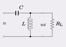
Figure 6. RLC circuit equally a low-pass filter	Figure 7. RLC circuit as a loftier-laissez passer filter
Figure eight. RLC excursion as a series band-pass filter in serial with the line	Figure 9. RLC circuit equally a parallel band-pass filter in shunt beyond the line
Figure 10. RLC circuit equally a series band-stop filter in shunt across the line	Figure eleven. RLC circuit as a parallel band-end filter in series with the line

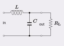
In the filtering application, the resistor becomes the load that the filter is working into. The value of the damping gene is called based on the desired bandwidth of the filter. For a wider bandwidth, a larger value of the damping cistron is required (and vice versa). The 3 components requite the designer three degrees of freedom. Two of these are required to fix the bandwidth and resonant frequency. The designer is still left with one which can be used to calibration $R$ , $50$ and $C$ to user-friendly practical values. Alternatively, $R$ may exist predetermined by the external circuitry which volition employ the terminal degree of liberty.

Low-pass filter [edit]

An RLC excursion can be used as a low-pass filter. The circuit configuration is shown in Figure half dozen. The corner frequency, that is, the frequency of the 3 dB point, is given by

\omega _{\mathrm {c} }={\frac {1}{\sqrt {LC}}}\,.

This is also the bandwidth of the filter. The damping factor is given past^[27]

\zeta ={\frac {1}{2R_{L}}}{\sqrt {\frac {L}{C}}}\,.

High-pass filter [edit]

A high-laissez passer filter is shown in Figure seven. The corner frequency is the same equally the low-pass filter:

\omega _{\mathrm {c} }={\frac {1}{\sqrt {LC}}}\,.

The filter has a stop-band of this width.^[28]

Band-pass filter [edit]

A band-pass filter can be formed with an RLC circuit past either placing a series LC excursion in series with the load resistor or else by placing a parallel LC circuit in parallel with the load resistor. These arrangements are shown in Figures 8 and nine respectively. The centre frequency is given by

\omega _{\mathrm {c} }={\frac {1}{\sqrt {LC}}}\,,

and the bandwidth for the series excursion is^[29]

\Delta \omega ={\frac {R_{L}}{L}}\,.

The shunt version of the circuit is intended to be driven past a high impedance source, that is, a constant current source. Nether those conditions the bandwidth is^[29]

\Delta \omega ={\frac {1}{CR_{Fifty}}}\,.

Band-end filter [edit]

Figure 10 shows a band-stop filter formed by a series LC circuit in shunt across the load. Figure 11 is a band-stop filter formed past a parallel LC excursion in series with the load. The first case requires a loftier impedance source so that the current is diverted into the resonator when it becomes low impedance at resonance. The second case requires a low impedance source then that the voltage is dropped across the antiresonator when it becomes high impedance at resonance.^[xxx]

Oscillators [edit]

For applications in oscillator circuits, it is generally desirable to make the attenuation (or equivalently, the damping factor) as small equally possible. In practice, this objective requires making the excursion's resistance $R$ as small equally physically possible for a serial circuit, or alternatively increasing $R$ to as much as possible for a parallel circuit. In either case, the RLC excursion becomes a good approximation to an platonic LC circuit. However, for very depression-attenuation circuits (high $Q$ -cistron), bug such as dielectric losses of coils and capacitors can become important.

In an oscillator circuit

\alpha \ll \omega _{0}\,,

or equivalently

\zeta \ll 1\,.

Every bit a effect,

\omega _{\mathrm {d} }\approx \omega _{0}\,.

Voltage multiplier [edit]

In a series RLC circuit at resonance, the electric current is limited only by the resistance of the circuit

I={\frac {V}{R}}\,.

If $R$ is small, consisting only of the inductor winding resistance say, then this electric current will be large. Information technology will drop a voltage beyond the inductor of

V_{L}={\frac {V}{R}}\omega _{0}L\,.

An equal magnitude voltage will also be seen across the capacitor but in antiphase to the inductor. If $R$ tin exist made sufficiently pocket-sized, these voltages can be several times the input voltage. The voltage ratio is, in fact, the $Q$ of the circuit,

{\frac {V_{Fifty}}{V}}=Q\,.

A like effect is observed with currents in the parallel circuit. Fifty-fifty though the circuit appears equally high impedance to the external source, there is a big current circulating in the internal loop of the parallel inductor and capacitor.

Pulse discharge circuit [edit]

An overdamped series RLC circuit tin can exist used as a pulse discharge circuit. Often information technology is useful to know the values of components that could exist used to produce a waveform. This is described past the class

I(t)=I_{0}\left(\,east^{-\alpha \,t}-due east^{-\beta \,t}\right)\,.

Such a circuit could consist of an energy storage capacitor, a load in the form of a resistance, some circuit inductance and a switch – all in serial. The initial conditions are that the capacitor is at voltage, $V 0$ , and at that place is no current flowing in the inductor. If the inductance $50$ is known, then the remaining parameters are given by the following – capacitance:

C={\frac {one}{~L\,\blastoff \,\beta \,~}}\,,

resistance (total of circuit and load):

R=50\,(\,\blastoff +\beta \,)\,,

initial terminal voltage of capacitor:

V_{0}=-I_{0}L\,\alpha \,\beta \,\left({\frac {1}{\beta }}-{\frac {one}{\alpha }}\correct)\,.

Rearranging for the case where $R$ is known – capacitance:

C={\frac {~\alpha +\beta ~}{R\,\alpha \,\beta }}\,,

inductance (total of excursion and load):

50={\frac {R}{\,\blastoff +\beta ~}}\,,

initial terminal voltage of capacitor:

V_{0}={\frac {\,-I_{0}R\,\blastoff \,\beta ~}{\alpha +\beta }}\left({\frac {one}{\beta }}-{\frac {i}{\alpha }}\right)\,.

See likewise [edit]

RC circuit
RL excursion
Linear circuit

References [edit]

^ Kaiser, pp. 7.71–vii.72.
^ "Resonant Circuits" (PDF). Ece.ucsb.edu . Retrieved 2016-10-21 .
^ Nilsson and Riedel, p. 308.
^ Agarwal and Lang, p. 641.
^ Agarwal and Lang, p. 646.
^ Irwin, pp. 217–220.
^ ^a ^b Agarwal and Lang, p. 656.
^ Nilsson and Riedel, pp. 287–288.
^ Irwin, p. 532.
^ Agarwal and Lang, p. 648.
^ ^a ^b Nilsson and Riedel, p. 295.
^ Humar, pp. 223–224.
^ Agarwal and Lang, p. 692.
^ Nilsson and Riedel, p. 303.
^ Irwin, p. 220.
^ This section is based on Example 4.ii.13 from Debnath, Lokenath; Bhatta, Dambaru (2007). Integral Transforms and Their Applications (2nd ed.). Chapman & Hall/CRC. pp. 198–202. ISBN978-1-58488-575-7. (Some notations have been changed to fit the rest of this commodity.)
^ Kumar and Kumar, Electric Circuits & Networks, p. 464.
^ Nilsson and Riedel, p. 286.
^ Kaiser, pp. v.26–five.27.
^ Agarwal and Lang, p. 805.
^ ^a ^b ^c ^d Cartwright, Thousand. Five.; Joseph, Eastward.; Kaminsky, E. J. (2010). "Finding the exact maximum impedance resonant frequency of a practical parallel resonant circuit without calculus" (PDF). The Technology Interface International Journal. eleven (1): 26–34.
^ Kaiser, pp. 5.25–5.26.
^ ^a ^b ^c ^d ^e ^f ^{one thousand} ^h Blanchard, Julian (October 1941). "The History of Electric Resonance". Bell System Technical Journal. USA: AT&T. twenty (four): 415. doi:10.1002/j.1538-7305.1941.tb03608.x. S2CID 51669988. Retrieved 2013-02-25 .
^ Savary, Felix (1827). "Memoirs sur l'Aimentation". Annales de Chimie et de Physique. Paris: Masson. 34: 5–37.
^ ^a ^b ^c ^d ^eastward Kimball, Arthur Lalanne (1917). A Higher Text-volume of Physics (2nd ed.). New York: Henry Concur. pp. 516–517.
^ ^a ^b ^c Huurdeman, Anton A. (2003). The Worldwide History of Telecommunications. USA: Wiley-IEEE. pp. 199–200. ISBN0-471-20505-2.
^ Kaiser, pp. 7.14–seven.xvi.
^ Kaiser, p. 7.21.
^ ^a ^b Kaiser, pp. 7.21–7.27.
^ Kaiser, pp. 7.30–7.34.

Bibliography [edit]

Agarwal, Anant; Lang, Jeffrey H. (2005). Foundations of Analog and Digital Electronic Circuits. Morgan Kaufmann. ISBN1-55860-735-8.
Humar, J. 50. (2002). Dynamics of Structures. Taylor & Francis. ISBNninety-5809-245-3.
Irwin, J. David (2006). Bones Engineering science Excursion Analysis. Wiley. ISBN7-302-13021-3.
Kaiser, Kenneth L. (2004). Electromagnetic Compatibility Handbook. CRC Press. ISBN0-8493-2087-9.
Nilsson, James William; Riedel, Susan A. (2008). Electric Circuits. Prentice Hall. ISBN978-0-13-198925-2.